How to increase or decrease values in excel without using formulas

Let's say you have to increase all the values in a worksheet to 10%. You can of course use a formula and multiply the value by 1.10. There is an alternate way, however, that you might like to use.
This will be useful specially when you need the new values without the formula. Use the excel paste special function. Yes, you've read it right,the paste special function!

Here's how to us this tool. First input the value in a cell, in this case the value 1.10. Copy this cell, then select all cells which contains the value to be changed and then right click. Choose paste special.

A dialog box will come up. Choose "multiply".

Click "OK". Now you're done! All your values are now 10% higher. All values are multiplied by 1.10. 

This can also be used to add, subtract, and divide the values by clicking the appropriate option buttons.

Happy computing!

Tweet

Excel through the years

Let's take a break from our excel tips and look a bit about microsoft excel history. Below are images of how previous versions of excel looked like. A trip down excel memory lane.

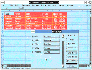
1987- Excel 2.0

1990 - Excel 3.0 

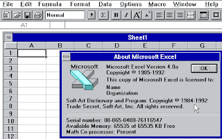
1992 - Excel 4.0

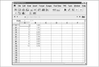
1993 - Excel 5.0

1995 - Excel for Windows 95 (version 7.0)

1997 - Excel 97

1999 - Excel 2000 (version 9.0)

May 31, 2001 - Excel 2002 (version 10.0)

October 21, 2003 - Excel 2003 (version 11.0)

November 30, 2006 - Excel 2007 (Version 12.0)

Excel 2010

There it is. Excel through the years! 

Tweet

Autosum shortcut

One of the most used formulas in excel is the sum function. Do you know that there is a shortcut that you can use to sum up a column or row of data aside from typing the =sum( ) function? Well, aside from clicking the autosum button , you can use this shortcut:

"Alt+="

It will automatically sum all the numbers for the rows or the column.

Try it.

Happy computing!

Tweet

5 Useful excel formulas for manipulating text

Excel has a lot of useful formulas for manipulating text. I'll cover some of the more useful ones. And most of which I often use.

1. Convert text to upper case.

    Excel has a function to convert text to all uppercase. And it is so easy, the formula is simply:

     =UPPER ("text")

    so to change a text in let's say A1, then just use =UPPER (A1). If cell A1 contains "excel", it becomes "Excel" on the cell with the formula.

   

2. Convert to proper case.

     Sometimes, you want to change to capital all the first letters of a phrase, sentence or group of words   such as titles. Here's a way to do this, use the formula:

   

   =PROPER("text")

  For example, if the text is "excel", then it becomes "Excel". If it is a sentence, a phrase, or group of words, it will capitalize the first letter of the first words. Example, "happy computing everyone" becomes "Happy Computing Everyone" (Quite useful for titles).

3. Extract left part of a text.

    If you want to extract part of a string then you can use this formula:

   =LEFT("text",number of letters)

  For example if cell A1 contains "ExcelEngineering" and you want only to get excel, then you can use this formula to extract "excel",

   =LEFT(A1,5)

   in other words, get 5 letters, starting from the LEFT from the text in A1..

4. Extract right part of a text.

    Very similar to the post above, but instead you start counting from the right.

   =RIGHT("text",number of letters)

   If cell A1 still contains "ExcelEngineering" and you want only to get "ring", then you can use this    formula to extract "ring",

   =RIGHT(A1,4)

   in other words, get 4 letters, starting from the RIGHT from the text in A1..

5. Extract anywhere in the text or string

   If you want to extract a text starting from any point in the string - not necessarily from the right or from the left, then use the function:

     =MID(text,position, number of letters)

  Using the same example of A1 with the word "excelegineering", if you want to extract the word   "engine", then use this formula:

    =MID(A1,6,6)

    in other words, start on the 6th letter of the text in A1(starting from the left) and get 6 letters.

 Happy computing!

Tweet

Add a Drop-Down List in Excel 2007,2010

Ever wondered how some worksheets have some drop-down list? Do you have to learn a very complicated macro or programming to do it on your own worksheet? Worry not, it is so easy. After learning this, you will be able to add this to your worksheet and make your worksheet look professional (and hopefully more user friendly). Here's the procedure.

1. Input all the data you want included in the drop-down list in a series of cells (example: A1:A5)
2. Click on the DATA tab in the ribbon
3. Select Data Validation
4. On the settings tab of the data validation dialog box, under "allow", choose list
5. Under the source box, input the list  of data (in this case A1:A5)
6. Now, you have a drop-down list. Well done!

Data validation on the ribbon

Data validation dialog box

Drop-down list in excel

            

               

Now, your worksheets will look more professional and you'll look more like an excel expert!

Happy Computing!

Tweet

Automatically Insert Current Time and Date in a Worksheet

If you want to display the current time and date in excel automatically, then just use this formula:

=Now()

This will return the current date and time in the format that you set in your windows preferences. If, on the other hand, you only want to see the date, then just use this formula:

=Today()


Here is a sample output of each formula:

Now()   : 5/21/2011 12:41
Today() : 5/21/2011



Happy Computing!

Tweet

How to use Excel VLOOKUP

One of my most used formula in excel is the VLOOKUP formula. Basically what this formula does is that it returns a certain value from a table given a specific value.

A very simple example would be like this.
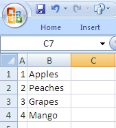
Assuming you have this table:

If you want to choose from the table given the number, then we can use VLOOKUP this way.

=Vlookup("1",A1:B4,2,False), this will result in "Apples"

In layman's terms, it means

=Vlookup("what to lookup for?", "what table?", "what column to get the results", "don't expect sorted data")

you can use a formula at the first argument to reference to another cell.

Now try it!

Happy Computing!

Tweet