5 Useful excel formulas for manipulating text

Excel has a lot of useful formulas for manipulating text. I'll cover some of the more useful ones. And most of which I often use.

1. Convert text to upper case.

    Excel has a function to convert text to all uppercase. And it is so easy, the formula is simply:

     =UPPER ("text")

    so to change a text in let's say A1, then just use =UPPER (A1). If cell A1 contains "excel", it becomes "Excel" on the cell with the formula.

   

2. Convert to proper case.

     Sometimes, you want to change to capital all the first letters of a phrase, sentence or group of words   such as titles. Here's a way to do this, use the formula:

   

   =PROPER("text")

  For example, if the text is "excel", then it becomes "Excel". If it is a sentence, a phrase, or group of words, it will capitalize the first letter of the first words. Example, "happy computing everyone" becomes "Happy Computing Everyone" (Quite useful for titles).

3. Extract left part of a text.

    If you want to extract part of a string then you can use this formula:

   =LEFT("text",number of letters)

  For example if cell A1 contains "ExcelEngineering" and you want only to get excel, then you can use this formula to extract "excel",

   =LEFT(A1,5)

   in other words, get 5 letters, starting from the LEFT from the text in A1..

4. Extract right part of a text.

    Very similar to the post above, but instead you start counting from the right.

   =RIGHT("text",number of letters)

   If cell A1 still contains "ExcelEngineering" and you want only to get "ring", then you can use this    formula to extract "ring",

   =RIGHT(A1,4)

   in other words, get 4 letters, starting from the RIGHT from the text in A1..

5. Extract anywhere in the text or string

   If you want to extract a text starting from any point in the string - not necessarily from the right or from the left, then use the function:

     =MID(text,position, number of letters)

  Using the same example of A1 with the word "excelegineering", if you want to extract the word   "engine", then use this formula:

    =MID(A1,6,6)

    in other words, start on the 6th letter of the text in A1(starting from the left) and get 6 letters.

 Happy computing!

Tweet

How to use Excel VLOOKUP

One of my most used formula in excel is the VLOOKUP formula. Basically what this formula does is that it returns a certain value from a table given a specific value.

A very simple example would be like this.
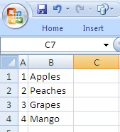
Assuming you have this table:

If you want to choose from the table given the number, then we can use VLOOKUP this way.

=Vlookup("1",A1:B4,2,False), this will result in "Apples"

In layman's terms, it means

=Vlookup("what to lookup for?", "what table?", "what column to get the results", "don't expect sorted data")

you can use a formula at the first argument to reference to another cell.

Now try it!

Happy Computing!

Tweet

Quick Auto Sum in Excel

Want to use a keyboard shortcut to quickly sum up a column or row of data? Here's how:

• Go to the end of the row or column (first cell with no values)
• Press Alt-= (Alt and equal sign)
• Auto sum is immediately inserted.
• Done!

Quick. Effective. Simple.

Happy Computing!

Tweet

Generate Random Numbers

There are two ways to generate random numbers in excel automatically:

1. Use the rand() function. It generates a random number from 0.1 to 0.9. To refresh just use F9. You can use "=round(rand()*100)" to generate whole numbers from 1 to 100. Or if you want, you can also use any other number as the multiplier.
2. Easier still, you can use "=RandBetween(a,b)". Where "a" and "b" are the least and max numbers that you want to generate. For example, if you want to generate a random number from 1 to 100. You will have to use =randbetween(1,100).
   
   Hope this helps!
   
   Happy computing!

Tweet

Finding a Maximum Value with a Condition ("MaxIF")

Very similar to last post. the "MinIf" function, if you want to get the maximum value with a condition then use this formula!

Assume data is in A1:A5 and want to get the maximum value BELOW 12,000, then.

=Max((if(A1:A5<12000,a1:a5,false))

Again, use CTL-SHIFT-ENTER to convert into an array formula and your done!

Tweet

Minimum Value Excluding Zero ("MinIf" function)

Ever confronted trying to find the minimum value excluding zero? Specially using downloaded metered data, there are times when you want to get the lowest value (with the exception of power interruption in which case it is zero). So how do we go about it in excel?

Here's the formula!

Assuming data is in cells E11-E18, then:

=MIN(IF(E11:E18>0,E11:E18,FALSE))

Basically, this formula says that, get minimum value IF the number in the array is greater than zero. If it is zero or below, do not consider it.

IMPORTANT NOTE: then instead of using only the enter key, use CTL-SHIFT-ENTER. This will convert the formula into an ARRAY FORMULA which will make this work. You can see if it is succesfully converted to array formula if you see a bracket enclosing the formula.

This formula can also be used with different conditions. This is one "MIN IF" formula.

Hope this helps! Note: You can also use this concept to create a "MAX IF" formula.

Tweet